geoFacets of Credit Quality

Published

January 2, 2023

obertwwalker.github.io

A GeoFacet View of Credit Quality

In previous work with Skip Krueger, we conceptualized bond ratings as a multiple rater problem and extracted measure of state level creditworthiness. I had always had it on my list to do something like this and recently ran across a package called geofacet that makes it easy to do. The end result should parse out state level credit risk and showcase the time series of credit risk for each of the states.

So here goes.

How’s that done?
library(haven)
library(dplyr)
library(geofacet)
Pew.Data <- read_dta(url("https://github.com/robertwwalker/academic-mymod/raw/master/data/Pew/modeledforprediction.dta"))
library(tidyverse)
load(url("https://github.com/robertwwalker/academic-mymod/raw/master/data/Pew/Scaled-BR-Pew.RData"))
state.ratings <- data.frame(state_name=Pew.Data$state, statefips=Pew.Data$statefips, year=Pew.Data$fyear, BR.Data)
state.ratings.long <- tidyr::gather(state.ratings, sampleno, value, -statefips, -year, -state_name)
state.SE <- state.ratings.long %>% group_by(state_name,year) %>% summarise(Credit.Quality=mean(value), t1=quantile(value, probs=0.025), t2=quantile(value, probs=0.975))
fips <-  data.frame(
stringsAsFactors = FALSE,
state_name = c("Alabama","Alaska","Arizona",
         "Arkansas","California","Colorado","Connecticut",
         "Delaware","Florida","Georgia","Hawaii","Idaho",
         "Illinois","Indiana","Iowa","Kansas","Kentucky","Louisiana",
         "Maine","Maryland","Massachusetts","Michigan",
         "Minnesota","Mississippi","Missouri","Montana","Nebraska",
         "Nevada","New Hampshire","New Jersey","New Mexico",
         "New York","North Carolina","North Dakota","Ohio",
         "Oklahoma","Oregon","Pennsylvania","Rhode Island",
         "South Carolina","South Dakota","Tennessee","Texas","Utah",
         "Vermont","Virginia","Washington","West Virginia",
         "Wisconsin","Wyoming","American Samoa","Guam",
         "Northern Mariana Islands","Puerto Rico","Virgin Islands"),
state = c("AL","AK","AZ","AR","CA",
                "CO","CT","DE","FL","GA","HI","ID","IL","IN","IA",
                "KS","KY","LA","ME","MD","MA","MI","MN","MS",
                "MO","MT","NE","NV","NH","NJ","NM","NY","NC","ND",
                "OH","OK","OR","PA","RI","SC","SD","TN","TX",
                "UT","VT","VA","WA","WV","WI","WY","AS","GU","MP",
                "PR","VI"),
fips = c("01","02","04","05","06",
         "08","09","10","12","13","15","16","17","18","19",
         "20","21","22","23","24","25","26","27","28",
         "29","30","31","32","33","34","35","36","37","38",
         "39","40","41","42","44","45","46","47","48",
         "49","50","51","53","54","55","56","60","66","69",
         "72","78"))  
Res1 <- left_join(state.SE, fips, by=c("state_name" = "state_name"))
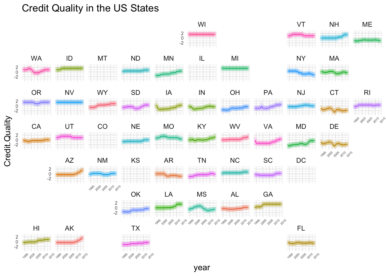
Plot1 <- Res1 %>% ggplot(., aes(x=year, y=Credit.Quality, group=state)) +
  geom_pointrange(aes(ymin=t1, ymax=t2, colour=state, fill=state), alpha=0.1) + 
  geom_line(aes(colour=state)) +
  guides(color="none", fill="none") +
  facet_geo(~ state) +
  theme_minimal() + 
  theme(axis.text.x = element_text(size=4, angle=45), axis.text.y = element_text(size=6)) + labs(title="Credit Quality in the US States")
Plot1

Not Long Ago I Learned

One thing that I quite liked about RMarkdown was column figures in the Tufte document templates. Those features are native to quarto, to a large extent. All we need do is add the following bit to code chunks.

#| column: margin
How’s that done?
Plot1

Figure 1: Credit quality in US States

Same with tables.

How’s that done?
knitr::kable(
  Res1[1:3, 1:3]
)
state_name year Credit.Quality
Alabama 1994 -0.3564650
Alabama 1995 -0.3576466
Alabama 1996 -0.3559865

References

How’s that done?
knitr::write_bib(names(sessionInfo()$otherPkgs), file="bibliography.bib")

References

Hafen, Ryan. 2020. Geofacet: Ggplot2 Faceting Utilities for Geographical Data. https://github.com/hafen/geofacet.
Müller, Kirill, and Hadley Wickham. 2022. Tibble: Simple Data Frames. https://CRAN.R-project.org/package=tibble.
Wickham, Hadley. 2016. Ggplot2: Elegant Graphics for Data Analysis. Springer-Verlag New York. https://ggplot2.tidyverse.org.
———. 2022a. Stringr: Simple, Consistent Wrappers for Common String Operations. https://CRAN.R-project.org/package=stringr.
———. 2022b. Tidyverse: Easily Install and Load the Tidyverse. https://CRAN.R-project.org/package=tidyverse.
———. 2023. Forcats: Tools for Working with Categorical Variables (Factors). https://CRAN.R-project.org/package=forcats.
Wickham, Hadley, Mara Averick, Jennifer Bryan, Winston Chang, Lucy D’Agostino McGowan, Romain François, Garrett Grolemund, et al. 2019. “Welcome to the tidyverse.” Journal of Open Source Software 4 (43): 1686. https://doi.org/10.21105/joss.01686.
Wickham, Hadley, Winston Chang, Lionel Henry, Thomas Lin Pedersen, Kohske Takahashi, Claus Wilke, Kara Woo, Hiroaki Yutani, and Dewey Dunnington. 2022. Ggplot2: Create Elegant Data Visualisations Using the Grammar of Graphics. https://CRAN.R-project.org/package=ggplot2.
Wickham, Hadley, Romain François, Lionel Henry, Kirill Müller, and Davis Vaughan. 2023. Dplyr: A Grammar of Data Manipulation. https://CRAN.R-project.org/package=dplyr.
Wickham, Hadley, and Lionel Henry. 2023. Purrr: Functional Programming Tools. https://CRAN.R-project.org/package=purrr.
Wickham, Hadley, Jim Hester, and Jennifer Bryan. 2022. Readr: Read Rectangular Text Data. https://CRAN.R-project.org/package=readr.
Wickham, Hadley, Evan Miller, and Danny Smith. 2022. Haven: Import and Export SPSS, Stata and SAS Files. https://CRAN.R-project.org/package=haven.
Wickham, Hadley, Davis Vaughan, and Maximilian Girlich. 2023. Tidyr: Tidy Messy Data. https://CRAN.R-project.org/package=tidyr.